Volume by Disc and Shell Methods

Volume by Disc and Shell Methods

6.3 Volume by slicing
6.4 Volume by shells

Note: Section numbers refers to Calculus, Early Transcendentals (2nd edition) by Briggs, Cochran, and Gillett.

These prints illustrate the disc method and the shell method for finding volumes of solids of  revolution.

The blue object is obtained by revolving the region between y-axis and the graph of:

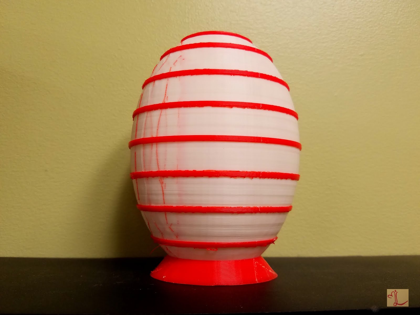
The model on the left shows the solid. The one on the right is an approximation using 10 shells.

In the solid below (titled the Volumes of Hanoi) the piece on the left of the model is a solid of revolution obtained by rotating the region bounded by the graph of the function 

The rightmost set of pieces represents an approximation of volume of the center solid of revolution with four discs, and the middle set represents a different approximation of that solid with four shells. The discs each have the same height but their radii are determined by the function f(x). The shells each have the same thickness but their heights are determined by the function f(x).

On one side is the approximation of the volume using four disks, and on the other side is the approximation of the volume using four shells. To make it clear which is which, we have shown the same model with the pieces taken apart.

The next model is a solid obtained by revolving the region between the graph of 

The model on the left is  the exact region, and the one on the right is an approximation which uses 8 shells.

Design credits: Shell approximation of solid of revolution I, mathgrrl, Apr 21, 2014, Shell approximation of solid of revolution II, mathgrrl, Apr 22, 2014, and Volumes of Hanoi, mathgrrl, Jan 18, 2014

Volume by slicing

Volume by slicing

Sec 6.3 Volume by slicing, Q10, pg 430 

Note: Section number refers to Calculus, Early Transcendentals (2nd edition) by Briggs, Cochran, and Gillett.

For this solid, it is possible to find the volume by integration of the cross sectional area. The solid has a circular base of radius r. The cross sections perpendicular to the base and parallel to the z-axis are equilateral triangles.  

The solid

Circular base

A sliced version so that it is possible to see the equilateral triangles:

 

Four slice version by Evelyn Sander.

The 20 slice version Volume: 20 equilateral triangles on circular base, dennedesigns, Jun 29, 2015. 

Double Integrals over Rectangular Regions

Double Integrals over Rectangular Regions


Section 13.1: Double Integrals over Rectangular Regions

Note: Section number refers to Calculus, Early Transcedentals (2nd edition) by Briggs, Cochran, and Gillett.

These 3D prints illustrate the concept of Riemann sums used for calculating volumes of solids. As the number of rectangles are increased, we get a better and better approximation of the double integral.

The double integral approximation for the function:

                                               

is demonstrated below. It is the Gaussian curve in 3 dimensions, generated using 100, 225, and 400 rectangular prisms, respectively on the interval [-2,2.5] x [-2,2]. The Mathematica code used to generate these models was based on Raouf Boules', Geoff Goodson's, Ohoe Kim's and Mike O'Leary's Calculus III Lab at Towson University, found here.

The integral approximator (code provided below) takes a function f on an interval [a1,b1]x[a2,b2] with n discretization points in both the x and y directions, therefore approximating the area under the function with n^2 rectangular prisms (cuboids in Mathematica). Just like in the 1-dimensional integral approximation methods, 

   

The x and y coordinates of the jth and kth rectangle are thus given by, 

Technical Details for Printing:


In Mathematica, Cuboid[{lower corner (x,y,z), upper corner (x,y,z)]. Here the lower corner is given by (x_j, y_k, 0), and the upper corner (x(j+1), y_(k+1), f(x_j, y_k)).

Mathematica code:

RD[f, {a1, b1}, {a2, b2}, n] := Show[Table[Graphics3D[Cuboid[{a1 + (b1 - a1)/nj, a2 + (b2 - a2)/nk, 0},

{a1 + (b1 - a1)/n(j + 1), a2 + (b2 - a2)/n(k + 1),f[a1 + (b1 - a1)/nj, a2 + (b2 - a2)/nk]}]], {j, 0, n - 1}, {k,0, n - 1}]]

Clear[f, x, y]

f[x, y] := 2*Exp[-x^2 - y^2]

print1 = RD[f, {-2, 2.5}, {-2, 2}, 10]

Export["filename.stl",print1]

In the figure below, from left to right, we have n=10, 15, 20 and 50.

This code was created by Mae Markowski, in Mathematics through 3D Printing, taught by Dr. Evelyn Sander in Spring 2016, and printed at the Math Makerlab, GMU. 

Klein Bottle

Klein Bottle







Model credits: Voronoi Klein Bottle, MadOverlord, Sep 3, 2013

Volume by Cross Section

Volume by Cross Section

6.3 Volume by slicing

Note: Section numbers refers to Calculus, Early Transcendentals (2nd edition) by Briggs, Cochran, and Gillett.

These prints illustrate a solid whose base is the region bounded by

The cross sections perpendicular to the base and parallel to the x-axis are squares. 

While it is possible to find the volume of this shape by via a cross section integral formula without ever visualizing it, it is a more satisfying experience if it is clear what it  looks like. 

Model credits: UNCC Calculus 2, Janthefischer, January 11, 2016

.

Saddle

Saddles

12.1 Planes and surfaces
12.2 Graphs and level curves
12.6 Directional derivatives and the gradient
12.8 Maximum/minimum problems

Note: Section numbers refers to Calculus, Early Transcendentals (2nd edition) by Briggs, Cochran, and Gillett.

Two saddles and a monkey saddle

Saddle surface

Saddle with grid lines and saddle with level sets

Here are two difference versions of a quartic surface: a standard mathematical saddle surface. This surface is the graph of the function 

In the red and blue version, the red curves second color depicts the level sets of the surface.  In the blue and white version, the blue curves depict the fixed x and fixed y grid lines. This point (x,y,z) = (0,0,1) (the middle point) is a critical point, meaning all partial derivatives are zero, but the point is neither a maximum nor a minimum. 

Monkey Saddle

The following print illustrates the graph of the function

This is a cubic surface. Like the standard saddle, it still has a critical point at (x,y) = (0,0), (the center), but it is even flatter than the standard saddle. It is called a monkey saddle since a monkey could sit on this saddle with room for both legs and its tail. 

Technical Details for Printing

These objects were designed in Mathematica. These technical notes were determined by trial and error (or more accurately error and error and error ad nauseam)

• The parametrization lines are created using the Tube command in Mathematica.
• This was printed with neither raft nor supports. 
• The blue base piece is needed in order to make the print work without falling over, the thickness of the white surface is 2, and the thickness of the blue parametrization is 2.5.
• In order to make the blue base pieces, I made spheres in Mathematica and used the hole options in Tinkercad to cut off the bottom half. Do not just leave the sphere intact and assume that the printer will ignore the part below the build plate. This actually seems to stop the printer for a long time and set there thinking about printing the bottom half of the sphere.
• Do not try to print something too steep - it seems that if it's about the same height as length and width you'll be better off. A steep piece can break off the base under its own weight. On the other hand, too wide will give the dreaded overhangs of more than 45 degrees.
• The side walls that are printed on the dual print can topple over. This seems to be a build plate adhesion problem. No consistent solution to this problem.

Quartic Surface with Level Sets

The saddle surface with level sets is made much the same as above, but the tubes are used for fixed height levels. 

Technical Details for Printing the monkey saddle

The standard monkey saddle function does not include the 1/2, but this made for too steep a figure, which started to break off at the corners. 

Paraboloid

Paraboloid

12.1 Planes and surfaces

12.2 Graphs and level curves
14.6 Surface integrals

Note: Section numbers refers to Calculus, Early Transcendentals (2nd edition) by Briggs, Cochran, and Gillett.

The surface defined by the equation

is a Paraboloid. The following 3D print shows a polar coordinate parameterization of a portion of the paraboloid above the xy-plane.

The horizontal curves are the z-level sets. They are all are ellipses, and in the special case a=b, they are circles. 

The parametrization is given by 

 

Thus the horizontal curves are curves of fixed z, and the vertical curves are curves of fixed t. 

Ellipsoid

Ellipsoid

12.1 Planes and surfaces

12.2 Graphs and level curves
14.6 Surface integrals

Note: Section numbers refers to Calculus, Early Transcendentals (2nd edition) by Briggs, Cochran, and Gillett.

The surface defined by the equation

is an Ellipsoid. Here are the level sets of constant height. The level sets are ellipses - hence the name of the shape!

The following object shows a polar parameterization of an ellipsoid given below with the parameters t and z. This surface can be used in discussion of parametrization of surfaces. The horizontal curves are curves of fixed z. The vertical curves represent the fixed t.