Wednesday, April 13, 2016

Level Sets


MATH 493: Math Through 3D Printing
Level Sets
Anneliese Slaton

“"Well, then, if a Point by moving three inches, makes a Line of three inches represented by three; and if a straight Line of three inches, moving parallel to itself, makes a Square of three inches every way, represented by three-to-the-second; it must be that a Square of three inches every way, moving somehow parallel to itself (but I don't see how) must make Something else (but I don't see what) of three inches every way—and this must be represented by three-to-the-third.’”

- Edwin. A. Abbot, Flatland: A Romance of Many Dimensions              


The challenge of representing n-dimensional objects (when n > 3) in a 3D space is one that has plagued the work for centuries. Mathematicians have been studying four-dimensional space since the time of Lagrange to present day.
One way to represent 4D space is to utilize level sets, a concept taught in multivariable calculus. Consider a function f(x,y,z). It is impossible to draw this, as it resides in 4D space. So instead, we choose a constant c to set f(x,y,z) equal to - this allows us to work in three dimensions, while observing how the function changes as c varies.
A level set is a real-valued function of the form
Lc(f) = {(x1, …, xn) | f(x1, …, xn) = c}.

To help us visualize a 4D graph, I printed the level sets of f(x,y,z)=exyz with four c values: c = 1, e, e2, e3. The level sets were then placed on the same graph. To print, they were connected with a series of supports through the centers of each graph piece.

Since f is differentiable, the level sets are hypersurfaces and, outside of the critical point of f at (0, 0, 0), they are manifolds (topological spaces that locally resemble Euclidean space).  Additionally, because f is differentiable, we know that the gradient of f at some point x is either 0 or perpendicular to the level set at the same point x.
Level sets can be used in the Level Set Method, a method that utilizes level sets for numerical analysis of surfaces and shapes.

The object to be printed was created using Mathematica and OpenScad for the supports. It was printed on the Makerbot 5th Generation 

printer. 


Sources:

Friday, April 8, 2016

Mandelbrot and Julia Sets


------------------------------------------

------------------------------------------

------------------------------------------

------------------------------------------

------------------------------------------


------------------------------------------

------------------------------------------


Wednesday, April 6, 2016

Chaotic Attractors

The following projects were created for GMU Math 493: Mathematics Through 3D Printing. They represent chaotic attractors. The prints themselves are hanging on a wind chime in the Math Department Office in Exploratory Hall, 4th Floor.


Chaotic Attractor Wind Chime


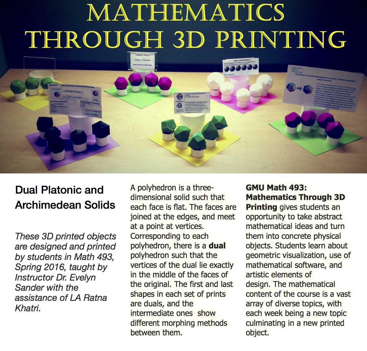
Duality of Platonic and Archimedean Solids

The following projects were created for GMU Math 493: Mathematics Through 3D Printing. They represent duality of solids. They are displayed in the math department display case in the atrium of Exploratory Hall (to the left as you enter).


A game of chaos

Written by Student C as part of Math 493: Mathematics Through 3D Printing

Let's play a game. A math game. A game... of chaos.

Heres how to play. Start out half-way (1/2) on our favorite interval [0,1]. Now flip a coin, heads move half way to 1 (¾), if tails move halfway to 0 (¼).

So now there were two outcomes- you are now either at ¾ or ¼. In either case, flip a coin. Lets say you are at 1/4- Heads, move half-way to 1 (5/8). Tails, move half-way to 0 (1/8). Now, if you were at 3/4 – Heads, move half-way to 1 (7/8). Tails, move half-way to 0 (3/8).

Do this a few more times to create your picture.

Now comes the time for reflection- if I say that you can do this as many times as you want, will you ever reach 0 or 1? What about ½? What about any of the points you received? That is, for every point that you've created, do you think that you will ever be able to get that number back by continuing to play this game? Remarkably, even if you play this game 100 times, 10,000 times, 100,000,000 times or even an infinite number of times, you will never be able to get back to any numbers that you've already created.

In this manner, we have discovered a set of numbers that have what is known as “measure 0”. That is, even though after doing this game an infinite number of times and generating a infinite number of numbers, the 'distance' to any two numbers is 0. That is, you cant play the game enough times to get back to any original number.
Now lets try extending this game. Let play this in 3 dimensions. Instead of looking at the two points on the number-line, lets look at the eight points on the unit cube. This game has to be slightly altered to play properly. First, number the points of the cube. Then, instead of flipping a two-sided coin, flip an 8 sided coin. When you flip the corresponding point, move half-way there. Again, do this as many times as you would like. Eventually, you will generate the Menger sponge. Several iterations of this can be viewed below:


Returning to this concept of measure 0, how does this apply to the Menger Sponge? Doing this iterative process an infinite number of times generates some interesting results. Namely, the volume of the entire object is zero. But perhaps, the more interesting notion is that the surface area is infinite. This can application can be “explored” by moving around “inside” the sponge, only to come to the conclusion that there is no way to ever find purchase of the object. In this way we can never reclaim any of the numbers we've generated. That is, measure 0 in 3 dimensions.


Sierpinski Triangle in 3 Dimensions

Sierpinski Triangle in 3 Dimensions

Mae Markowski
April 5, 2016


The following post is by Mae Markowski as a part of George Mason University
Math 493, Mathematics Through 3D Printing.

We will examine the 3-dimensional Sierpinski Triangle, Sierpinski tetrahedron, or Sierpinski pyramid, as it sometimes goes by. To begin, we will first examine the Sierpinski triangle in 2 dimensions, the multiple ways in which it is created, and then see the simplest way to generate the figure in 3-dimensions. Lastly we will take a look at the final 3D-printed model and
the code which led us there.

The Sierpinski triangle is what is known in general as an iterated function system. These are fractal, or self-similar in nature, meaning that you can zoom in as far as you want and you would keep seeing the same thing again and again. It received its namesake after Polish mathematician Waclaw Sierpinski,  but has been around since well before Sierpinski. The triangle is formed in several ways. Easiest to grasp is the method of removing triangles.For instance, start with an equilateral triangle, cut it into 4 equal triangles, remove the center triangle, and repeat. In this way for n iterations we have
3n cells in our figure. (The cells being the smallest of the triangular units.) Below is an image after n = 3 iterations. Here, it is more clear that we will in the infinite limit remove an area of value 1, but still have infinitely many points in our set. Thus, this is a Cantor set.


More interestingly, the same triangle can be drawn via the Chaos Game, a game that one would guess is random, but actually always leads us to this self-similar pattern. Addtionally, this set also has the relationship that it is modulus 2 of Pascal’s Triangle. Because the third creation method is slightly more complicated, we will focus on the first method as we move to 3D. In 3 dimensions, we now no longer have planar cells in our shape. Each cell is now a pyramid. So in our first iteration, when we remove one pyramid from the middle, we are left with 4 cells leftover. Similarly, for n = 2, we have now 16 units. In general, after n iterations, there will be 4n cells left in the object, the extra dimension reflected in the increase of our base number being raised to the n power.

The code used to generate the Sierpinski pyramid in OpenSCAD constructs equilateral triangles, and then appropriately assigns vertices of the ones remaining after n iterations. The pyramids for n = 2; 3; 4; 5 are shown below
Because at 5 iterations we are already at 45 units in our pyramid, I opted to print out the cases of n = 1; 2; 3; 4, which are shown below. Also worth noting is that these objects were printed with supports. Because the n = 4 has so many cells that it has to print, I would think supports are necessary; however, you always run the risk of not being able to get them off. Thus, the pictures below still have the supports intact.
These were printed using the Makerbot 5th Generation. If interested in having your own, there are many other models up on Thingiverse. If interested in more of the mathematical models, the following links can further your reading:


Fun with Fractals


Fun with Fractals

By Hope Roberts
George Mason University
Math 493
Mathematics through 3D Printing

What are Iterated Functions & Fractals?

Iterated functions are a way of constructing Fractals.
An iterated function  takes a function  X → X and composes another function of itself a repeated amount of times. (Wikipedia).
Repeating the same function over and over is known as iteration.
After so many iterations the structure is seen to shrink. This is known as limiting behavior. The set will converge to a single fixed point, which is known as the attractive fixed point.

Example of a self-similar repeating pattern.

Fractals are patterns that repeat infinitely. The patterns repeated are complex and self-similar. The repeated patterns are created by recursion, so repeating a pattern in a similar way.


Brief History on Iterated Functions

Iterated functions are credited to John E Hutchinson discovered in 1981.
Michael Barnsley’s is credited with making them popular in a book he wrote titled Fractals.


Making of my Fractal

Using OpenSCAD with code given by Dr. Sander I changed the design of the Fractal by adjusting the set of  rules of the fractal, specifically changing r, s and theta in the code. Changing the r,s and theta of the code by any amount yielded a different shape.
I obtained these values from a yale.edu (reference at bottom)
The type picked from this website was (o).


Original structure before the code was adjusted.

I then adjusted the length and width in the code so that the platform and bases were supporting the structure in such a way that the printing would have support in all areas of the structure. Finally I added one additional layer of height to the structure from 5 levels to 6 levels also increasing the height of each layer, which increased the thickness of each layer.


My Fractal after adjustments to r,s, theta, length, width and height.


In MakerBot I adjusted the size to a four-hour approximate time for printing, making sure the structure was flat on the surface with supports and rafts.

Equations & Code Changes:

Below is the basic equation for an iterated function.

if for all components of  f, it is in X

Below are my values for r, s and theta for my Fractal:

scale1x = -.5; scale2x = .5; scale3x = .5;  scale1y = .5; scale2y = .5; scale3y = .5;  theta1  = 90;  theta2 =  -90; theta3 =  0;

Below are my values for the changes to length, width and height in my code.

len = 45; // length of the first segment wid = 45; // width of the first segment height  = 3.0; // height of the first cube.

Finished Product:


The finished product was successful and there was relatively no clean up of the structure involved.


Sources: