Saddle

Saddles

12.1 Planes and surfaces
12.2 Graphs and level curves
12.6 Directional derivatives and the gradient
12.8 Maximum/minimum problems

Note: Section numbers refers to Calculus, Early Transcendentals (2nd edition) by Briggs, Cochran, and Gillett.

Two saddles and a monkey saddle

Saddle surface

Saddle with grid lines and saddle with level sets

Here are two difference versions of a quartic surface: a standard mathematical saddle surface. This surface is the graph of the function 

In the red and blue version, the red curves second color depicts the level sets of the surface.  In the blue and white version, the blue curves depict the fixed x and fixed y grid lines. This point (x,y,z) = (0,0,1) (the middle point) is a critical point, meaning all partial derivatives are zero, but the point is neither a maximum nor a minimum. 

Monkey Saddle

The following print illustrates the graph of the function

This is a cubic surface. Like the standard saddle, it still has a critical point at (x,y) = (0,0), (the center), but it is even flatter than the standard saddle. It is called a monkey saddle since a monkey could sit on this saddle with room for both legs and its tail. 

Technical Details for Printing

These objects were designed in Mathematica. These technical notes were determined by trial and error (or more accurately error and error and error ad nauseam)

• The parametrization lines are created using the Tube command in Mathematica.
• This was printed with neither raft nor supports. 
• The blue base piece is needed in order to make the print work without falling over, the thickness of the white surface is 2, and the thickness of the blue parametrization is 2.5.
• In order to make the blue base pieces, I made spheres in Mathematica and used the hole options in Tinkercad to cut off the bottom half. Do not just leave the sphere intact and assume that the printer will ignore the part below the build plate. This actually seems to stop the printer for a long time and set there thinking about printing the bottom half of the sphere.
• Do not try to print something too steep - it seems that if it's about the same height as length and width you'll be better off. A steep piece can break off the base under its own weight. On the other hand, too wide will give the dreaded overhangs of more than 45 degrees.
• The side walls that are printed on the dual print can topple over. This seems to be a build plate adhesion problem. No consistent solution to this problem.

Quartic Surface with Level Sets

The saddle surface with level sets is made much the same as above, but the tubes are used for fixed height levels. 

Technical Details for Printing the monkey saddle

The standard monkey saddle function does not include the 1/2, but this made for too steep a figure, which started to break off at the corners. 

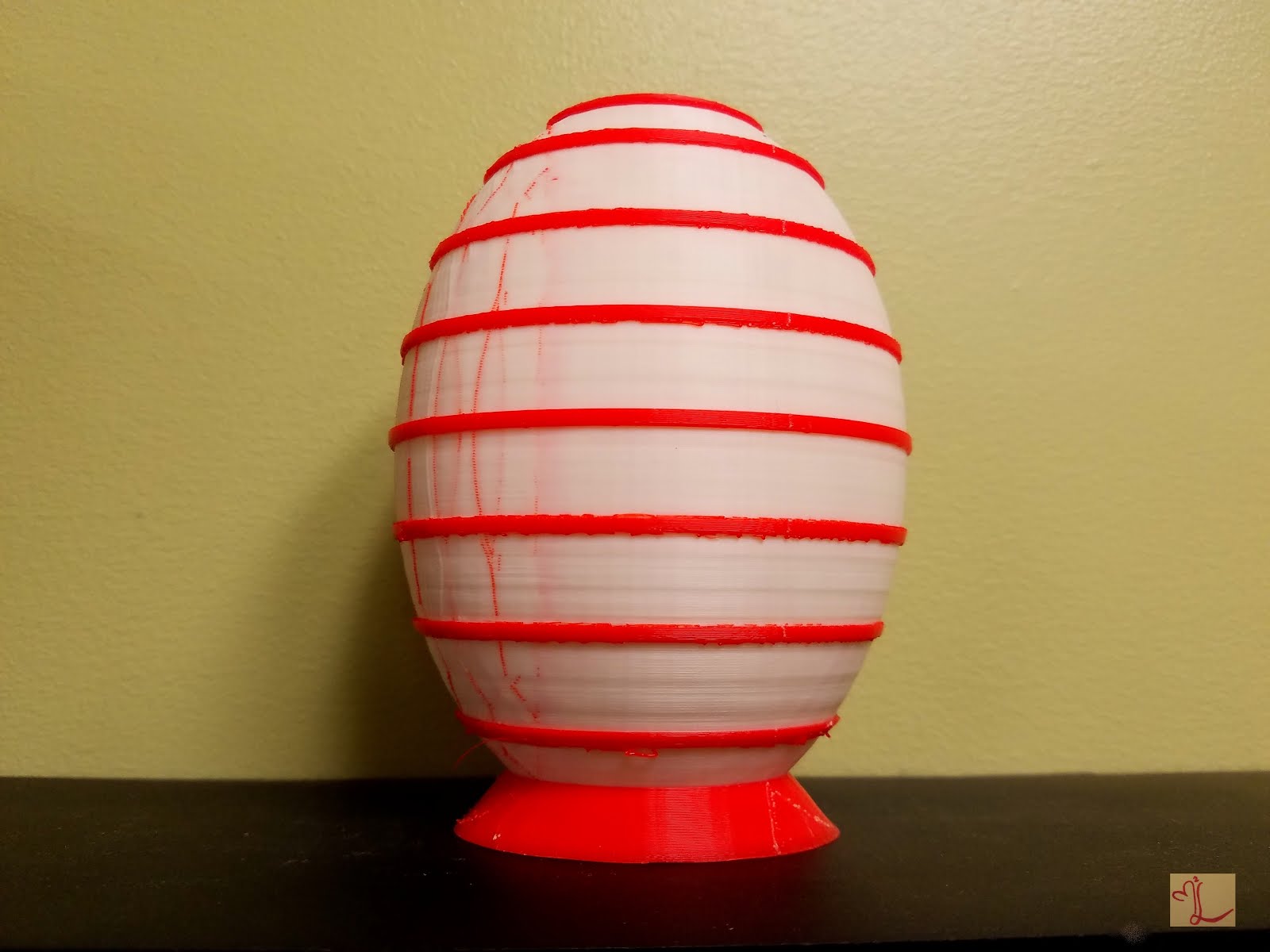
Paraboloid

Paraboloid

12.1 Planes and surfaces

12.2 Graphs and level curves
14.6 Surface integrals

Note: Section numbers refers to Calculus, Early Transcendentals (2nd edition) by Briggs, Cochran, and Gillett.

The surface defined by the equation

is a Paraboloid. The following 3D print shows a polar coordinate parameterization of a portion of the paraboloid above the xy-plane.

The horizontal curves are the z-level sets. They are all are ellipses, and in the special case a=b, they are circles. 

The parametrization is given by 

 

Thus the horizontal curves are curves of fixed z, and the vertical curves are curves of fixed t. 

Ellipsoid

Ellipsoid

12.1 Planes and surfaces

12.2 Graphs and level curves
14.6 Surface integrals

Note: Section numbers refers to Calculus, Early Transcendentals (2nd edition) by Briggs, Cochran, and Gillett.

The surface defined by the equation

is an Ellipsoid. Here are the level sets of constant height. The level sets are ellipses - hence the name of the shape!

The following object shows a polar parameterization of an ellipsoid given below with the parameters t and z. This surface can be used in discussion of parametrization of surfaces. The horizontal curves are curves of fixed z. The vertical curves represent the fixed t. 

Discontinuous Surface with Parabolic Contours

Discontinuous Surface with
Parabolic Contours

12.3 Limits and continuity

Note: Section numbers refers to Calculus, Early Transcendentals (2nd edition) by Briggs, Cochran, and Gillett.

This function is discontinuous at (x,y)=(0,0). The limit of f(x,y) along every straight line through the origin is 0 (as shown for the three lower yellow curves). However, the function has a different limit along every parabola through the origin - as shown by the upper yellow curve. In fact, the parabolas through the origin are exactly the level sets of the surface. 

Discontinuous Surface

Discontinuous Surface

12.3 Limits and continuity

Note: Section numbers refers to Calculus, Early Transcendentals (2nd edition) by Briggs, Cochran, and Gillett.

A function of two (or more) variables is continuous at a point, provided its limit equals its value at that point.
The function

is discontinuous at (x,y)=(0,0). 

The graph is a surface of fixed height along each line through the origin - a very hard concept to wrap the mind around. This creates the fold in the middle. Note in the print below that there are four fixed height lines (in purple) to emphasize this strange fact. 

The title of this post reflects the fact that the graph looks very much like a specialty pasta (See http://recipes.wikia.com/wiki/File:Funghini.jpg).

Tangent Space of Twisted Cubic

Tangent Space of a Twisted Cubic

A twisted cubic is the curve  . This is a smooth, rational curve C of degree three in projective 3-space P3. It is a fundamental example of a skew curve. It is essentially unique, up to projective transformation (the twisted cubic, therefore). It is generally considered to be the simplest example of a projective variety that is not linear or a hypersurface, and is given as such in most textbooks on algebraic geometry. It is the three-dimensional case of the rational normal curve, and is the image of a Veronese map of degree three on the projective line.

(Information obtained from Wikipedia).

This design was created by Conor Nelson in Mathematics through 3D Printing, taught by Dr. Evelyn Sander in Spring 2016, and printed at the Math Makerlab, GMU. 

GMU News Coverage

Students use 3-D printers to transform mathematical equations into art