Sierpinski Pentagon

Sierpinski Pentagon

Savannah Crawford

MATH401 - Fall 2019

This object is the Sierpinski Pentagon. It's similar to the Sierpenski Triangle in construction. It is generated by an iterated function system that scales down five pentagons and translating them to the corners. The scaling factor is (3 - 5^(-1/2))/2. The Sierpinski Pentagon is the limiting set for this construction. 

Here is the code that generated the print: 

And here is the generated preview of the STL:

This object shows the Sierpinksi pentagon iterated four times, with an unscaled pentagon at the base layer to hold everything together. openSCAD could only handle up to 4 iterations of the function, beyond that the rendering took an unreasonably long time and the resulting STL was not printable.

Here is the completed object: 

The object was printed with a MakerBot Z18 and tough PLA filament. For a print with dimensions of approximately 20cm x 20cm x 5cm, it took a little over 8 hours. The print was successful at the scale, but since the top layer has very thin pentagons, it may be unsuccessful.  

The object is not a perfect Sierpenski Pentagon because the pentagons are not perfectly aligned with the corners of the preceding pentagon.  For future printing, I would work to correct this. It is also difficult to see the multiple layers of the of the iterated functions, so for a future print I would also print every other layer in a contrasting color so this is easier to see. 

These images are cool because they make it easier to see the multiple layers:

Duality of Platonic Solids

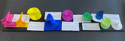
These representations of the duality of platonic solids were created jointly with Arsah Rahman and Patrick Bishop, and never got their proper photo in this blog. Cube/octahedron duality in red/blue. Icosahedron/dodecahedron duality in purple/yellow. And tetrahedron self-duality in green/yellow.

Data Visualization Prints

Using 3D printing for data visualization gives and opportunity to express individual interests and background.

Andros Island

Colston DiBlasi

MATH 401; Mathematics Through 3D printing 

November 18, 2019

Data Visualization

Andros Island

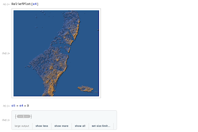
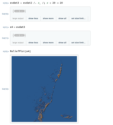
For this assignment I went about it a different way. I used the topographical map of the Bahamas. I was curious if water level rises how does it affect how the Bahamas. At the beginning of the assignment I attempted to do all of the Bahamas. This was a mistake because they are so spread out and some are very small it was hard to see all of the islands. What I ended up doing was just looking at the big island in the Bahamas called Andros Island. I took the topographical graph and I cut off the depth, so the lowest point was 0 which is at sea level. I did this because off of the Bahamas is the Marian Trench which is over 6000 feet deep. Then I decided to look at if current water levels rise then by 2200 the water level would rise about 20 feet. From this information I then made the cut off at 20 feet. This allowed me to see what the Bahamas would look like if the water level was 20 feet higher. I then printed both of these so you could compare how much of Andros Island in the Bahamas would be lost if the water level rose 20 feet. 

This is the code for the normal Island:

The codes all the same but then you just change this one line of code. You change 0 -> 0 to 20 -> 20:

When writing the code to print some struggles that I encountered the majority of my problems. The main problem that I encountered was when trying to figure out how to get the thickness increases. This was a problem because I need to get a base to print it on. When I printed the current water level it took about 3.5 hours. The increased water level only took 1 hour and 15 min. This is what my final prints looked like.

Total Fertility Rate in Asia

Pantea Ferdosian

MATH 401; Mathematics Through 3D printing 

November 18, 2019

Data Visualization

Total Fertility Rate is Asia

            For this assignment, I printed an illustrative model of Fertility Rate (TFR) of all the countries in Asia. The total fertility rate (TFR), sometimes also called the fertility rate, absolute/potential natality, period total fertility rate (PTFR), or total period fertility rate (TPFR) of a population is the average number of children that would be born to a woman over her lifetime if:

·      She was to experience the exact current age-specific fertility rates (ASFRs) through her lifetime, and

·      She was to survive from birth to the end of her reproductive life.

It is obtained by summing the single-year age-specific rates at a given time.(Wikipedia)

Also, according to the Population Reference Bureau, Total Fertility Rate (TFR) is defined as, “the average number of children a women would have assuming that current age-specific birth rates remain constant throughout her childbearing years.” Simply put, total fertility rate is the average number of children a woman would have if a she survives all her childbearing (or reproductive) years. Childbearing years are considered age 15 to 49.

The model displayed here shows how Total fertility rate varies by country. The different heights of the countries correspond to the magnitude of the indicator. The taller the height, the higher the value.

I designed this print using the “prism” function that was given in the sample document and got the data through “TotalFertilityRate” command on Mathematica. The source for all the data that I used in this assignment is: Wolfram Research, Inc., SystemModeler, Version 12.0, Champaign, IL (2019).

Nested Platonic Solids

This set of the five nested platonic was designed by Jack Love and  Evelyn Sander in 2015. However, for some strange reason, no image ever appeared on this blog to record it.

Strange Chaotic Attractors

Visualizing Strange Chaotic Attractors

These 3D printed objects are designed and printed by students in Math 401, Fall 2019, taught by Instructor Dr. Evelyn Sander with the assistance of Chloe Ham and Colin Chung.

Chaotic solutions for differential equations 

Solutions to 3-dimensional systems of differential equations can be quite simple, such as a point that never moves, or a periodic motion that repeats forever. It can also be quite complicated, such as these prints. Each is a solution to a differential equation which is a 

Strange:  the object has interesting fractal shapes with many gaps 

Chaotic:   for two nearby initial conditions, solutions will move away from each other  

Attractor: any nearby initial condition has a solution limiting to the shape you see

Riemann surface prints ready for display

Visualizing Riemann Surfaces

These 3D printed objects are designed and printed by students in Math 401, Fall 2019, taught by Instructor Dr. Evelyn Sander with the assistance of Chloe Ham and Colin Chung.

Graphing functions in the complex  plane

The complex plane is  two-dimensional, meaning that the graph of complex functions are four dimensional. We cannot see in four dimensions, so we project to three dimensions. This gives a sense for what the these graphs  look like in 4D. 

Arneodo System

Chaos

In mathematics most things can be predicted quite simply if enough information is provided. This though doesn’t apply to the chaotic system, as in their names are quite chaotic and are difficult to predict. Some examples of this in real world would be the weather. We have developed systems to be able to predict it to some extent but it can vary from initial prediction, this is the basis of butterfly effect that initial condition can vary the final result greatly. The other simple example is a double pendulum, depending on where it is dropped it would result in much different results.

            What we did was look at different attractors that would create different systems. In essence attractors are set of numeric values to which a system tends to evolve from. If these values are to be slightly changed it would result in a complete different and non-chaotic system. To have the system figured out over longer and longer periods it would need to be integrated. The reason to find these attractors is to be able to recognize and to eliminate them to help with models.    

            The system looked at today is called an Arneodo system. Visually it can be though as two reflexive disk that have an extension in the middle but seeing the visual it self is much better. To get the model has to be referred from thermohaline convection and reduction of its partial differential equations to an ordinary differential equation, this would result in Arneodo. 

            Initial conditions that are found for the formula are system can be seen in the image. The system it self for the most part can be seen quite simple but does result in quite bizarre shape. And these models can be quite hard to do by hand but are usually performed with computers to help model them but still that is very limited to what they look long term.

            As can be seen the chaos is quite complex though we are able to mitigate it a bit with these attractors. In long term it is impossible to predict how these things will end up looking like and we are only able to get some sense with the attractors. There are many more of these chaotic maps, some that are complex, and are one dimension.

Illia Stadnyk